During the peak of the accounting busy season, the influx of closing tasks can be overwhelming.

Annually, Quarterly or Monthly closing have attacked the accountant non-stop. In the midst of this chaos, I sought a way to reclaim my time.

To build a solution where complex bookkeeping data can be converted and prepared for posting with a single click—turning hours of manual work into a one-second refresh.”

🚀 Let’s explore together ! 🚀

🧩 Tools – Power Query

🧩 Task – To unpivot data to perform in accounting format record

📖 Input and Output data.

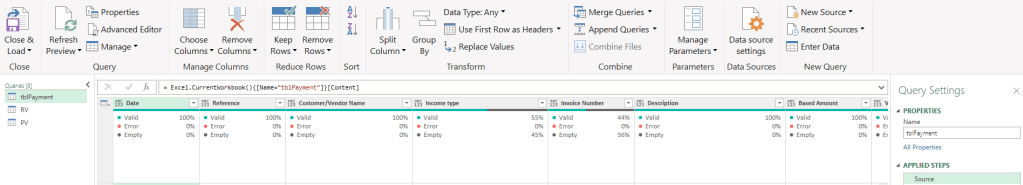
This is the input data.

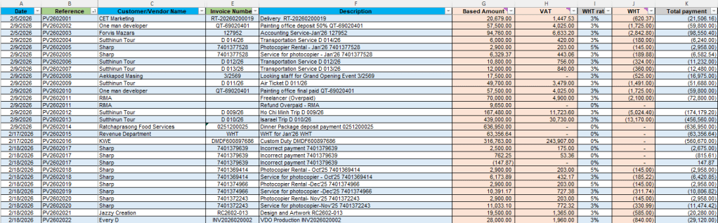
Source data is recorded by horizontal format. However in the bookkeeping way we need to transpose column G , H and J into rows to categorize them into accounting format (Debit and Credit)

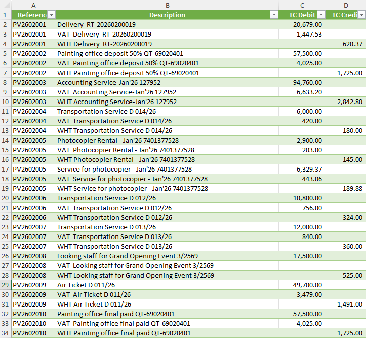
This is the output that we want.

📖 How to transform the data.

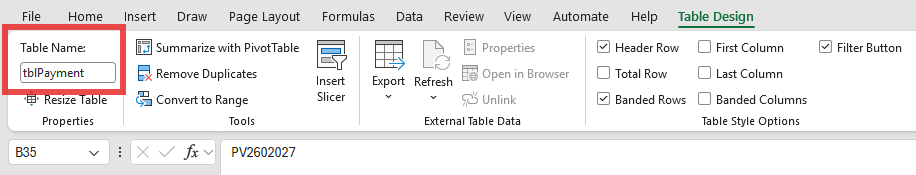
The raw data (input) need to transform it to table when we add transactions it will automatically update in Power Query.

Covert range to table by Crtl+T then name it

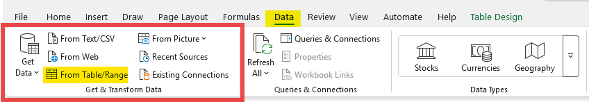
then, get data to connect with power query.

Going to the ribbon > Data > Get & Transform data from Table/Range

🚀 Welcome to the world of power query. Let’s prep data !!!

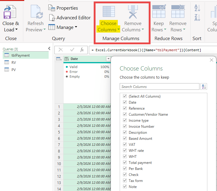
📌 1. Remove un-using column by Home > Manage columns “Choose Columns” then uncheck the column that we want to remove.

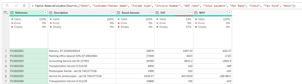
💥Boom – here is the result💥

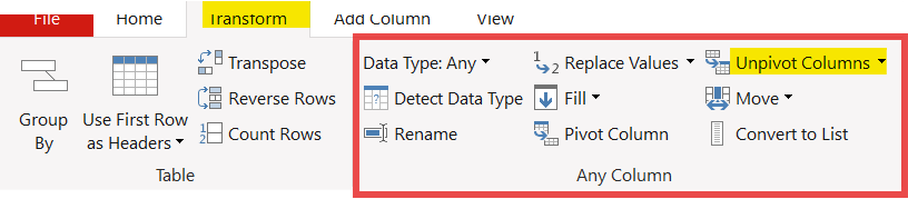
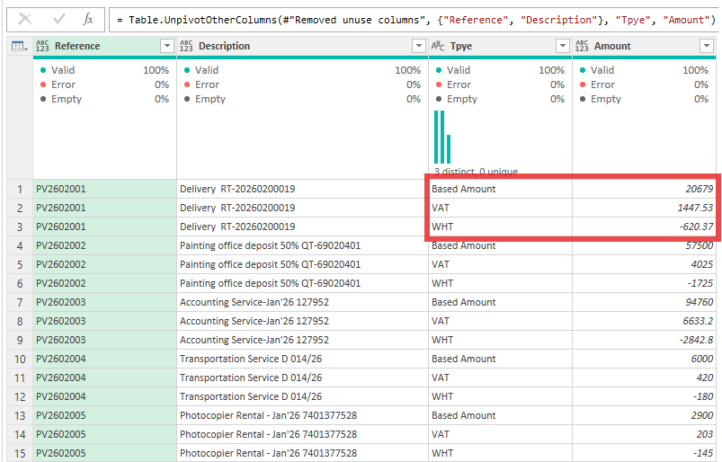
📌 2. Let’s unpivot column “Based amount, VAT and WHT” into rows by Transform > Any column “Unpivot columns”

💥Boom – here is the result💥

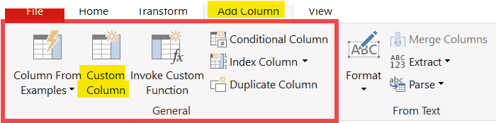
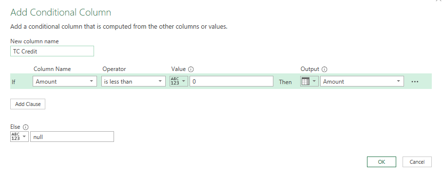
📌 3. Time to split positive and negative amount into the Debit/Credit columns (Positive = Debit , Negative = Credit) by Add column > General “Custom column” > Do it twice to extract separate columns.

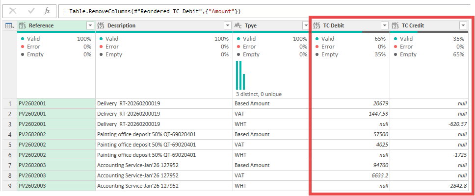
then clean un-using column and change data types

💥Boom – here is the result💥

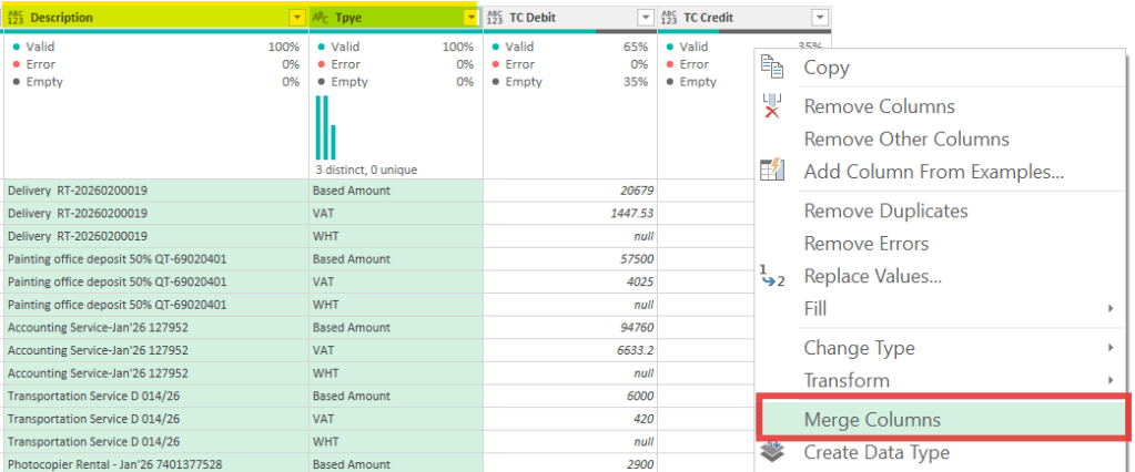
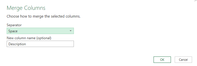
📌 4. To identify type of transactions, we need to create proper description so, merging column between Description + Type by Selecting column that we want to merge > right click “Merge Column.

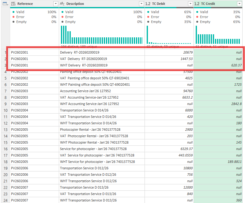
then clean data by trim data, change type and turn negative amount in column “TC credit” to positive amount.

💥Boom – here is the final result💥

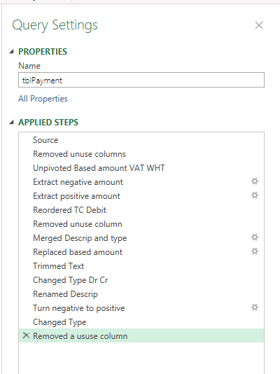
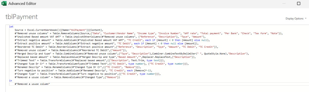
📖 The applied steps and M code.

🚀 Close and load go go go ~~

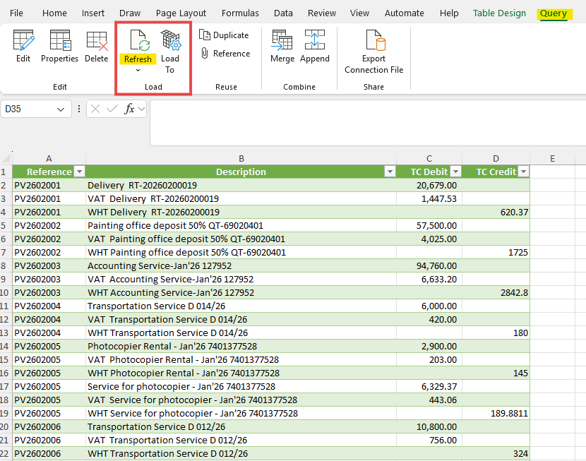
Here is the final output when your input table update,

Selecting the output worksheet in your excel file > go to Query tap > Press “Refresh” ✅

No need to copy paste any more 🤩

Hope you like the content like this.

Welcome to all feedback ✌️

Thank you and see you next week 🖤